library(tmap)
library(sf)Introduction
Why a map?
We love maps in WASH. Geo-location information is one of the most important type of data to collect and use. It helps to evaluate and monitor many aspects of WASH such as infrastructure planning or service access. To create and visualize such information on a map gives multiple benefits.
- Map is straight-forward. To understand how waste skips are distributed across a town, it is more intuitive to label the skips locations on a map instead of reading a long list of locations.
- Map is informative. To compare the concentration of humanitarian organizations globally, a thematic map can illustrate nicely by coloring the regions differently based on the concentration. To gain this insight from a table, however, needs multiple aggregation back and forth.
- Map is fun. To play around with a map is not a difficult job anymore. With a few lines in R, we can produce interactive WASH maps to communicate with a broad range of audience.
Useful R libraries
To create and visualize maps, we will need the help with the following R libraries to process geospatial data and plot the maps. We start with two useful libraries that will deliver a static map showing the locations:
sf: a package that supports “simple features” (an encoding of spatial data).tmap: a package that can quickly plot thematic maps.
There are other libraries that are commonly used to add external geodata (e.g, rnaturalearth) and make interactive plots (e.g., leaflet). You will learn more about them in the next blog posts.
Useful openwashdata datasets
Typically, a location point is described by its longitude and latitude. For this tutorial, we select two published datasets in openwashdata that collected geo-location data points.
wasteskipsblantyre: Data on locations of the publicly accessible waste skips in Blantyre, Malawi collected in 2021.cbssuitabilityhaiti: Spatial data to support an analysis of suitability of container-based sanitation in flood prone areas of Haiti.
Plot map with collected data
Preparation
- You have R and RStudio installed, or you can access Posit Cloud.
- You have programmed a few lines in R programming, and know how to run commands in the console window.
- You have installed and used R packages before.
- You have familiarity with geospatial data and terms, such as longitude, latitude, and coordinate reference system.
Package Installation
To install the above-mentioned R packages, run the following command in the console.
install.packages("sf", "tmap") To install an openwashdata R data package, for example, the `cbssuitabilityhaiti` package. Run the following command in the console. If you do not have the package devtools installed, you need to run the first line too.
# install.packages("devtools")
devtools::install_github("openwashdata/cbssuitabilityhaiti")
If you want to install another openwashdata R data package, you need to change the cbssuitabilityhaiti to the corresponding package name.
Basic thematic map
Now we have installed all needed R libraries. In the following sections, we will show two examples to create a quick view of the collected location data.
First, load the libraries.
1. Example: Waste skips in Blantyre, Malawi
library(wasteskipsblantyre) # Load the openwashdata R packageYou could get a taste of the dataset by looking at the first a few rows of the data,
head(wasteskipsblantyre)
#>                   name     long       lat capacity_l
#> 1      Ndirande ground 35.05063 -15.77515       7000
#> 2 Chimwankhunda mosque 35.01484 -15.82705       7000
#> 3         Naizi market 35.08819 -15.84962       7000
#> 4    Machinjiri market 35.08105 -15.74466       7000
#> 5   South Lunzu market 35.05611 -15.73089       7000
#> 6         Khama market 35.07455 -15.76771       7000
Each row in the dataset wasteskipsblantyre is a geolocation of a waste skip. We focus on the columns long and lat to plot these skips. First, we need to convert the location columns into a format that is designed for geospatial data. To achieve this, we use the function st_as_sf from the sf package as the following:
sf_wsb <- st_as_sf(wasteskipsblantyre, coords = c('long', 'lat'), crs = 4326)We specify two parameters here, coords and crs. Because we are plotting points on the map, we need to tell what columns from our data holding these points (i.e. coordinates). In our case, we have seen that the column long and lat provide the longitude and latitude coordinates. Then, we need to give which coordinate reference system is used.
Now we can use this formatted geodata to plot a map showing waste skip locations.
sf_wsb |>
  tm_shape() + # a necessary step to tell a map will be created
  tm_dots() + # plot the locations
  tm_graticules() # create coordinate grid lines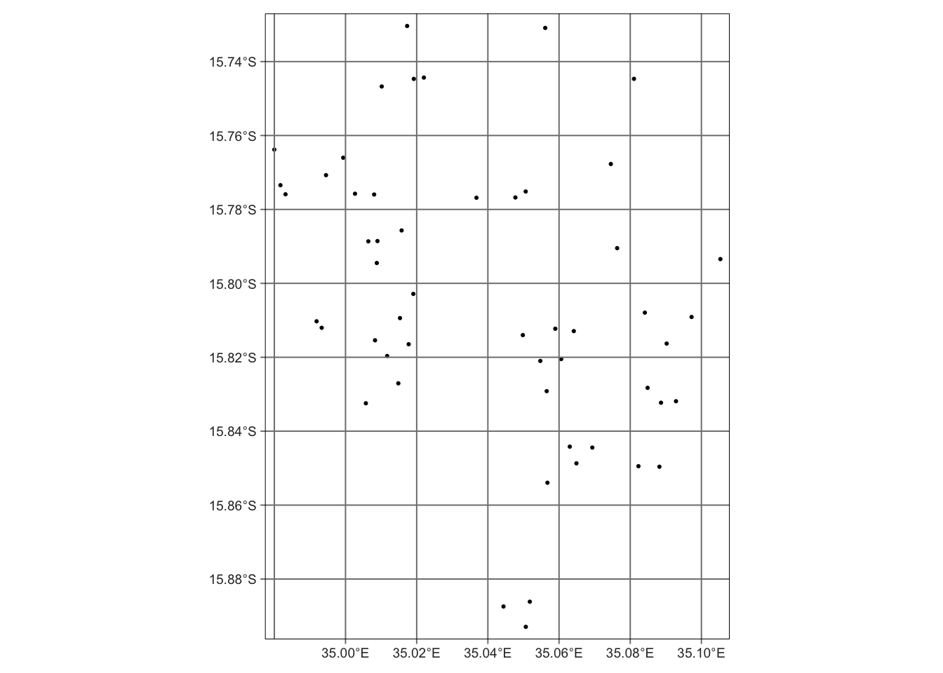
If you are interested in knowing more about the dataset, check out this amazing tutorial: https://openwashdata.github.io/wasteskipsblantyre/articles/examples.html
2. Example: Water access in Cap Haïtien, Haiti
You might notice that the first example only shows the locations rather than locations on top of a base map, such as the city map. This is because the data does not include the geospatial information about the city, for example, the boundaries between districts. You will learn how to combine with external data to resolve this in the next post. Now, what if we also collected data to plot the base map?
In this example, the dataset contains both water access points (in mwater) as well as the base map geometry (in okap) for the municipality of Cap Haïtien. As before, we can plot the water access points like:
library(cbssuitabilityhaiti)

mwater|> tm_shape() +
    tm_dots() +
    tm_graticules()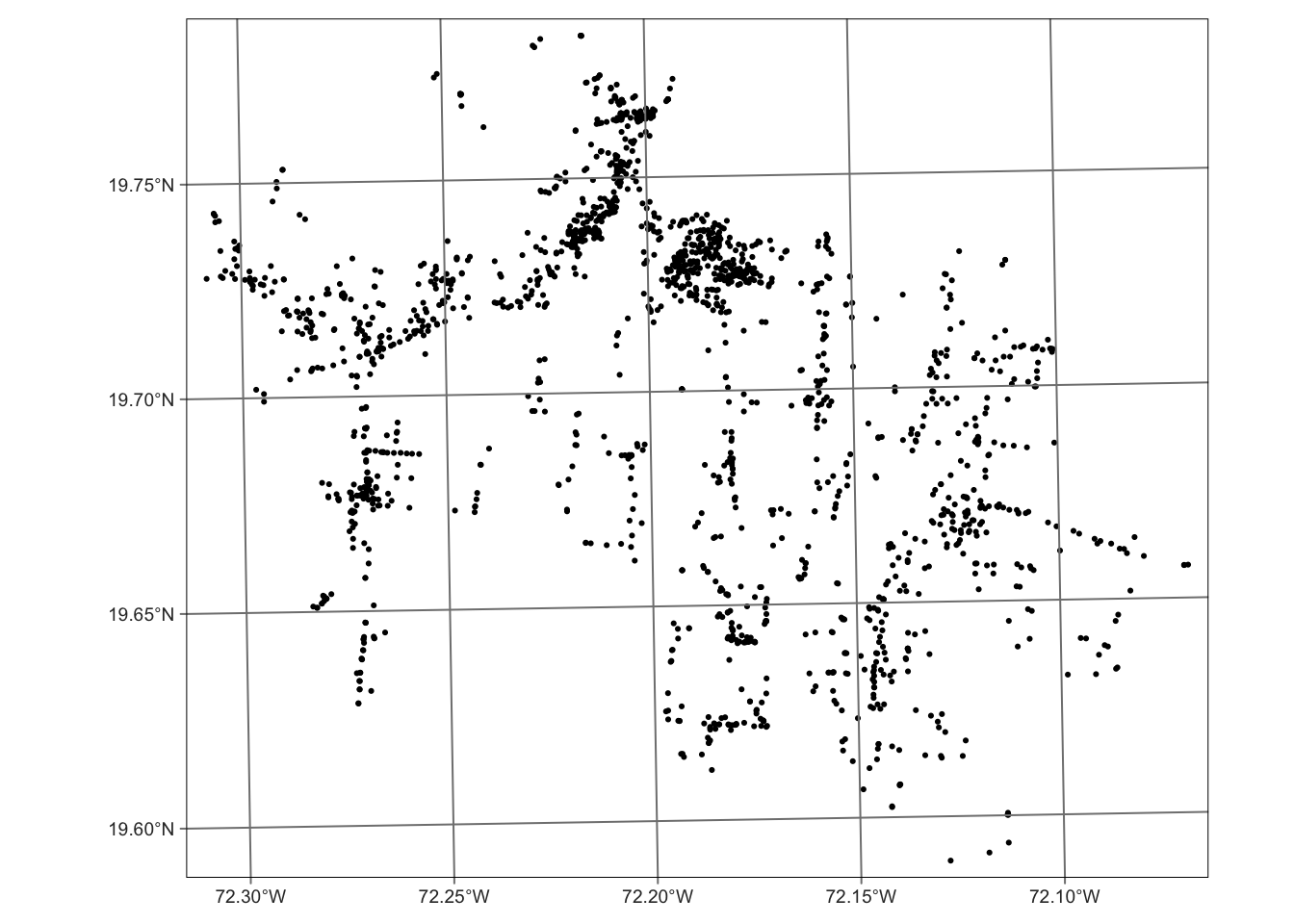
We can plot the base map from okap as the following:
okap |> tm_shape() +
    tm_borders() +
    tm_fill(alpha = 0.6) +
    tm_graticules()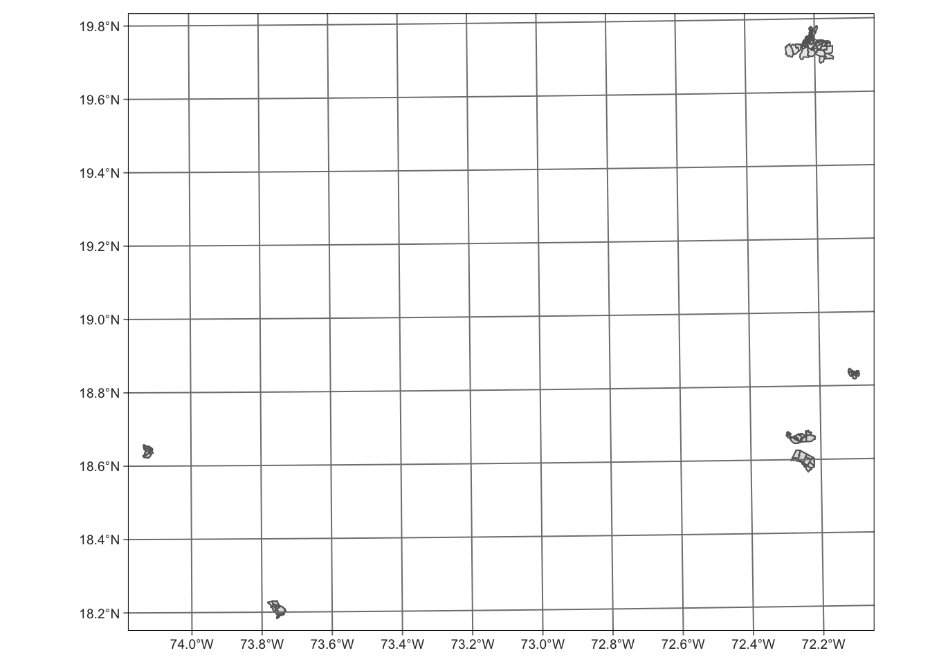
We can see that okap data contains more than Cap Haïtien data. Therefore, we need to filter the data okap on cte variable (Name of the communes) to keep data only relevant to Cap Haïtien before combining the two maps.
library(tidyverse)
caphaitien <- filter(okap, cte == "ctecaphaitien")

caphaitien |> tm_shape() +
    tm_borders() +
    tm_fill(alpha = 0.6) +
    tm_graticules()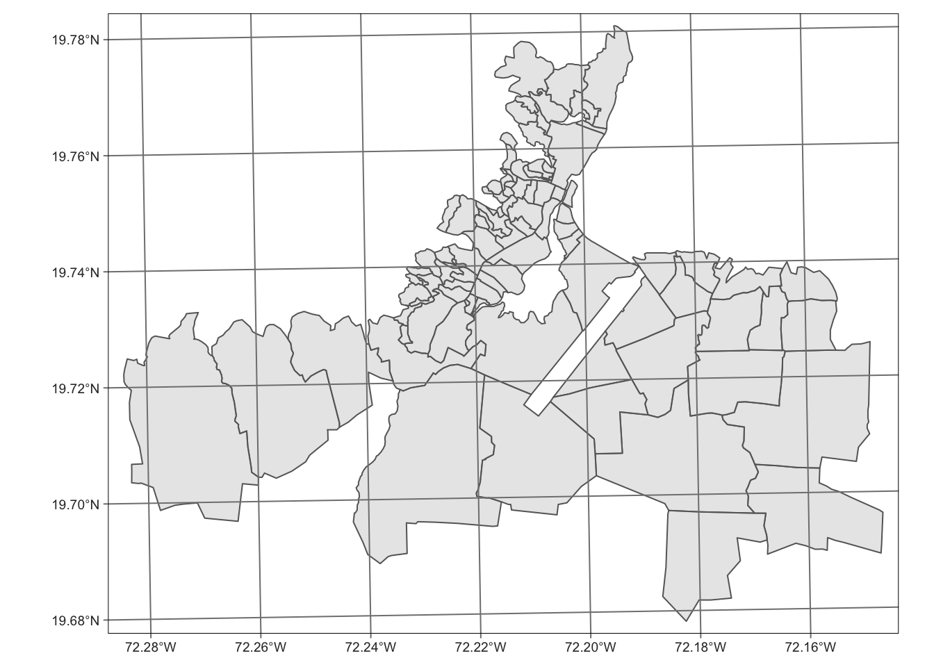
Now, let’s see what happens if we stack these two map layers together.
# Create base map layer
tm_shape(caphaitien) +
    tm_borders() +
    tm_fill(alpha = 0.6)  +
  # create second map layer: locations of the water points
    tm_shape(mwater) +
    tm_dots() +
    tm_graticules()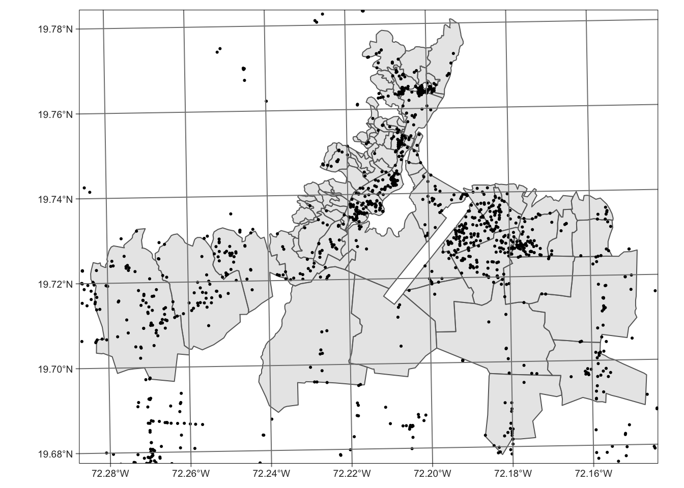
This is still a little problematic. Many water points are plotted outside of the base map.The base map may not contain enough boundary information to cover all areas where certain water points were recorded. One way is to join the two datasets to include water points within the base map area. We might also want to remove the coordinate gridlines for better visuals.
We join join the base map data to mwater data and remove observations that do not have a unique identifying number neighborhood unit. Note: joining map data takes order into account, st_join(caphaitien, mwater) would render different results.
# Join the data and filter
caphaitien_join <- st_join(mwater, caphaitien) |> drop_na(neighborho)

# Create base map layer
tm_shape(caphaitien) +
    tm_borders() +
    tm_fill(alpha = 0.6)  +
  # create second map layer: locations of the water points
    tm_shape(caphaitien_join) +
    tm_dots()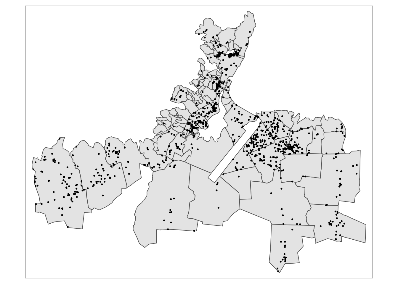
Finally, we can visualize other features about the water points by adding parameters in tm_dots(). For example, we can color different types of the water points as follows:
# Create base map layer
tm_shape(caphaitien) +
    tm_borders() +
    tm_fill(alpha = 0.6)  +
  # create second map layer: locations of the water points
    tm_shape(caphaitien_join) +
    tm_dots(col = "type")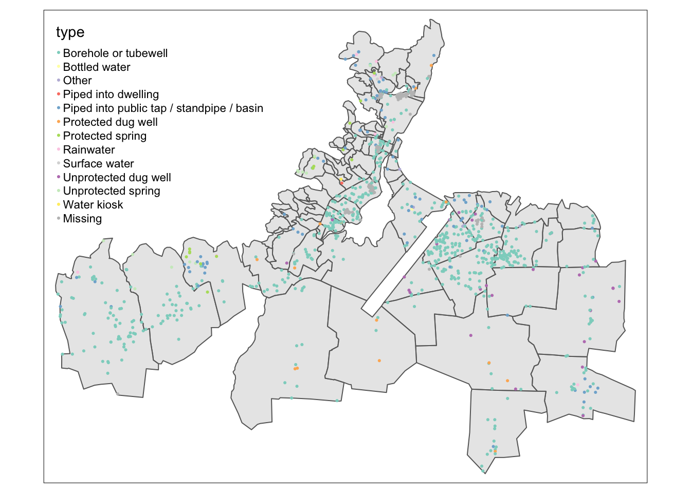
If you are interested in knowing more about this dataset, we have a wonderful detailed tutorial: https://openwashdata.github.io/cbssuitabilityhaiti/articles/examples.html
What’s next?
- Plot maps with external geospatial data
- Make an interactive map
References: